Overview

Problem Statement

We investigate the distribution of the longitudinal magnetic field component along the axis of a multi-coil solenoid.

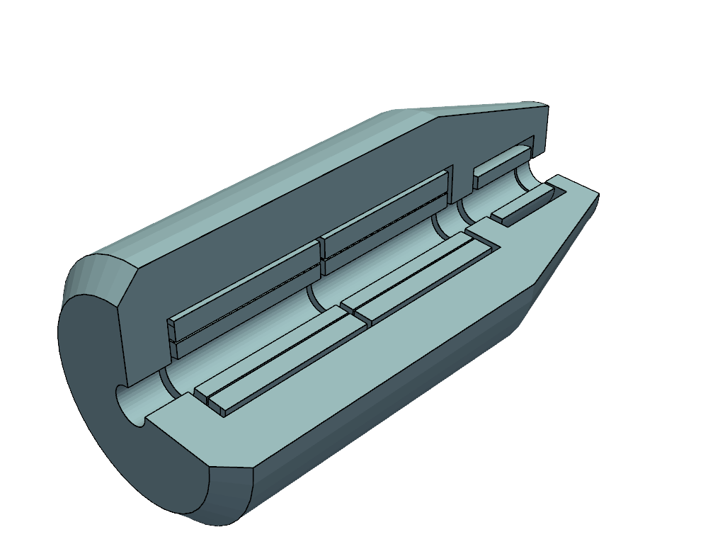
Five concentric current-carrying coils are arranged inside an iron yoke. The entire assembly possesses axial symmetry. We need to find the distribution of the longitudinal magnetic field component along the axis of the system and the integral of this component.

Schematically, the domain under investigation appears as follows:

The magnetic permeability values of all materials are known throughout the domain. The coils are characterized by their number of turns and current. The three-dimensional geometry is shown below.

Mathematical Formulation

The fundamental mathematical model used to simulate nearly all macroscopic electromagnetic phenomena is the Maxwell equations system, which relates the electric and magnetic field components, medium parameters (electrical conductivity, magnetic and dielectric permittivity), and external sources of electromagnetic fields in the form of a system of vector differential equations:

$$\nabla\textbf{H} = \textbf{J}^{ext} + \sigma\textbf{E} + \frac{\partial(\varepsilon\textbf{E})}{\partial t}, \\ \nabla\textbf{E} = \frac{\partial\textbf{B}}{\partial t}, \\ \nabla\textbf{B} = 0,\ \nabla(\varepsilon\textbf{E}) = \rho,$$

where $\textbf{H}$ is the magnetic field intensity, $\textbf{J}^{ext}$ is the external current density vector, $\textbf{E}$ is the electric field intensity, $\sigma$ is the specific electrical conductivity of the medium, $\varepsilon$ is the dielectric permittivity of the medium, $\textbf{B}$ is the magnetic flux density (related to the field intensity $\textbf{H}$ by $\textbf{B} = \mu\textbf{H}$, where $\mu$ is the magnetic permeability coefficient).

The task of magnetostatics refers to modeling the magnetic field created by a stationary (constant) electric current with a known distribution density $\textbf{J}$. Such fields are described by two equations from the full Maxwell system:

$$\nabla\textbf{H} = \textbf{J}, \\ \nabla\textbf{B} = 0.$$

Description of Stationary Magnetic Fields Using the Vector Potential

We represent $\textbf{B}$ as the curl of some vector-valued function $\textbf{A}$, called the vector potential: $\textbf{B} = \nabla\textbf{A}$.

With this representation of $\textbf{B}$, Gauss’s equation becomes the identity $\nabla(\nabla\textbf{A}) = 0$, and the vector potential can be obtained from Ampère’s equation, where $\textbf{H} = \mu^{-1}\textbf{B} = \mu^{-1}\nabla\textbf{A}$:

$$\nabla(\frac{1}{\mu}\nabla\textbf{A}) = \textbf{J}.$$

In the axisymmetric case, the current density vector has only one non-zero component $J_{\phi}$, and both $J_{\phi}$ and the magnetic permeability $\mu$ are independent of the $\phi$ coordinate: $J_{\phi} = J_{\phi}(r, z)$, $\mu = \mu(r, z)$. In this case, the magnetic field is completely determined by only one component $A_{\phi}$ of the vector potential $\textbf{A}$, satisfying the two-dimensional equation

$$-\nabla(\frac{1}{\mu}\nabla A_{\phi}) + \frac{1}{\mu}\frac{A_{\phi}}{r^2} = J_{\phi}$$

or in cylindrical coordinates:

$$-\frac{1}{r}\frac{\partial}{\partial r}(\frac{r}{\mu}\frac{\partial A_{\phi}}{\partial r}) - \frac{\partial}{\partial z}(\frac{1}{\mu}\frac{\partial A_{\phi}}{\partial z}) + \frac{A_{\phi}}{\mu r^2} = J_{\phi}.$$

We perform the variable substitution

$$u(r, z) = rA_{\phi}(r, z)$$

and transform the resulting equation:

$$A_{\phi} = \frac{u}{r}$$ $$\frac{\partial A_{\phi}}{\partial r} = \frac{1}{r}\frac{\partial u}{\partial r} - \frac{u}{r^2},\ \frac{\partial A_{\phi}}{\partial z} = \frac{1}{r}\frac{\partial u}{\partial z}$$ $$\frac{r}{\mu}\frac{\partial A_{\phi}}{\partial r} = \frac{1}{\mu}(\frac{\partial u}{\partial r} - \frac{u}{r})$$ $$\frac{1}{\mu}\frac{\partial A_{\phi}}{\partial z} = \frac{1}{\mu r}\frac{\partial u}{\partial z}$$ $$\frac{A_{\phi}}{\mu r^2} = \frac{u}{\mu r^3}$$

Substituting these relations into the original equation and simplifying yields the following elliptic equation:

$$-\frac{\partial}{\partial r}(\frac{1}{\mu r}\frac{\partial u}{\partial r}) - \frac{\partial}{\partial z}(\frac{1}{\mu r}\frac{\partial u}{\partial z}) = J_{\phi}.$$

The field can be obtained from the following relations:

$$B_r = -\frac{1}{r}\frac{\partial u}{\partial z},\ B_z = \frac{1}{r}\frac{\partial u}{\partial r}.$$

Boundary Conditions

For the problem under consideration, the following boundary conditions are appropriate:

1. Axis condition:

$$r = 0 \rightarrow u = 0$$

2. Remote boundary condition (field decays):

$$u = 0,\ A_{\phi} = 0$$

The weak form will have a different appearance in this case, but after the variable substitution, the form reduces to that obtained above.

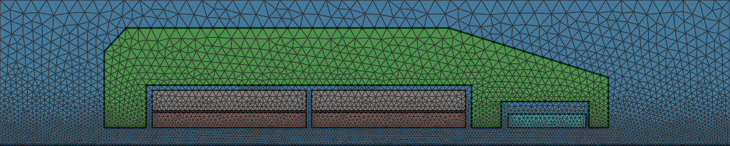
Finite Element Mesh

When constructing the finite element mesh, several important considerations must be addressed:

1. The domain must be partitioned into multiple physical groups;
2. The mesh refinement in the solenoid axis region must be significantly higher than outside the solenoid.

We use the open-source GMSH package for mesh generation.

Numerical Simulation

To solve the equation on the constructed mesh, we use the FEniCS computational platform for solving partial differential equations via the finite element method.

Weak Form Formulation

We introduce a test function $v \in V$, where $V = H_0^1(\Omega)$ (square-integrable functions with square-integrable gradient and zero value on the Dirichlet boundary).

Multiplying the original equation by $v$

$$-\nabla(\frac{1}{\mu r}\nabla u)v = J_{\phi}v$$

and integrating over the domain

$$\int_{\Omega}-\nabla(\frac{1}{\mu r}\nabla u)v d\Omega = \int_{\Omega}J_{\phi}v d\Omega.$$

Using Green’s formula and accounting for the zero value of the test function on the domain boundary, we obtain the weak form equation:

$$\int_{\Omega}\frac{1}{\mu r}\nabla u \nabla v d\Omega = \int_{\Omega}J_{\phi}v d\Omega.$$

Note that when deriving the three-dimensional axisymmetric case, the weight $r$ appears:

$$dV = rdrdzd\phi.$$

After integrating over $\phi$:

$$dV = 2\pi rdrdz.$$

Basis

To approximate the function $u$, and consequently $A$, we use a first-order continuous Galerkin functional space, which means applying piecewise-linear continuous basis functions on triangular elements.

Considering the form of the equation for the longitudinal field component

$$B_z = \frac{1}{r}\frac{\partial u}{\partial r}$$

numerical computation requires excluding the axis itself: $r \ne 0$. This can be achieved in two ways:

1. Use a zeroth-order discontinuous Galerkin space to approximate the field, i.e., describe the solution with piecewise-constant functions on each finite element.
2. When computing the field, exclude elements located on the axis. In this case, the same basis used for approximating the vector potential can be used to approximate the field.

For the current problem, the first variant was chosen since the mesh in the axis region is sufficiently fine, meaning piecewise-constant functions will describe the field with adequate accuracy. Additionally, the first approach does not require additional modifications to the approximation algorithm, significantly simplifying the final solution.

Software Implementation

When programmatically describing the variational form, we must account for the variation of physical parameters within the computational domain. For this purpose, each parameter (magnetic permeability and current) will be defined as piecewise-constant functions:

J = fem.Function(Q)
J.x.array[:] = 0.0
J.x.array[nbsn] = fem.Constant(data.mesh, (nbsn_n * nbsn_i) / nbsn_s)
J.x.array[nbti] = fem.Constant(data.mesh, (nbti_n * nbti_i) / nbti_s)
J.x.array[comp] = fem.Constant(data.mesh, (comp_n * comp_i) / comp_s)

mu0 = 4 * np.pi * 1e-7

mu = fem.Function(Q)
mu.x.array[air] = fem.Constant(data.mesh, mu0)
mu.x.array[iron] = fem.Constant(data.mesh, mu0 * 1000.0)
mu.x.array[nbsn] = fem.Constant(data.mesh, mu0)
mu.x.array[nbti] = fem.Constant(data.mesh, mu0)
mu.x.array[comp] = fem.Constant(data.mesh, mu0)

where $Q$ is the zeroth-order discontinuous Galerkin space:

Q = fem.functionspace(data.mesh, ('DG', 0))

The variational form, in this case, takes the simplest form:

u = ufl.TrialFunction(V)
v = ufl.TestFunction(V)
a = (1.0 / (mu*r)) * ufl.dot(ufl.grad(u), ufl.grad(v)) * ufl.dx
L = J * v * ufl.dx

where $V$ is the first-order continuous Galerkin functional space:

V = fem.functionspace(data.mesh, ('CG', 1))

The distribution of the longitudinal component is interpolated onto the space $Q$:

Bz = fem.Function(Q)
Bz.interpolate(fem.Expression((1.0 / r) * ufl.grad(uh)[1],
    Q.element.interpolation_points))

To compute the integral of the longitudinal component along the solenoid axis, we must declare a measure that includes first-order elements (line segments) located on the axis. In our case, such elements belong to the 8th physical group (this group was defined using GMSH during mesh generation). The integral is then computed as follows:

dz = ufl.Measure("ds", domain=data.mesh, subdomain_data=data.facet_tags)
I = fem.assemble_scalar(fem.form(Bz * dz(8)))

Result

As a result of measuring the magnetic field distribution, the integral of the longitudinal component on the solenoid axis is obtained:

$$\int_{Oz}B_z dz \approx 7.643\ T.$$

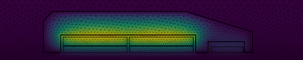
Vector Potential

The figure below shows the distribution of the r-weighted vector potential value $u = rA_z$:

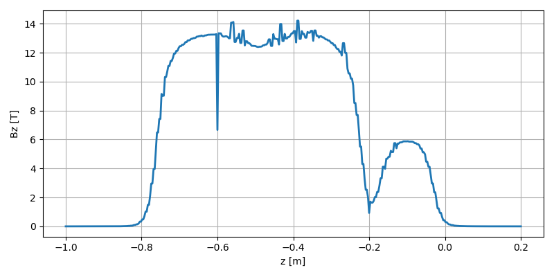
Longitudinal Component of Magnetic Flux Density

The following figure shows the distribution of the longitudinal component of magnetic flux density $B_z$:

---

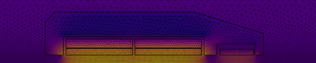
Field distribution along the axis:

Verification

To verify the correctness of the obtained result, we present the residual norm of the weak form:

$$||R(v)|| = ||a(u_h, v) - L(v)|| approx 6.314772 times 10^{-09}.$$

Additionally, we verify the correctness of global physical integrals, specifically the magnetic energy value (field method)

$$W_{B} = \int\frac{1}{2\mu}|B|^2 dV,$$

and compare it with the magnetic energy computed via the vector potential (source method)

$$W_{A} = \int J_{\phi}A_{\phi} dV.$$

After reducing the above expressions to cylindrical coordinates, we obtain

$$|W_{B} - W_{A}| approx 8.731149 times 10^{-11}.$$